
Well Logging Interpretation for Formation and Reservoir Properties Guide
1. Introduction
Electrical logging is a formation evaluation technique developed in the late 1920s by the brothers Conrad and Marcel Schlumberger, who introduced the first downhole Resistivity measurement in France, thereby formally establishing the concept of "wireline logging." The method was introduced to the United States in 1929 and, by the mid-1930s, had become widely adopted across the industry. Over the decades, Electrical Logging has evolved from simple Resistivity measurements into a comprehensive portfolio of downhole wireline measurements that now include Gamma Ray, Resistivity, Density, Neutron Porosity, Sonic, and other advanced tools.
Well‐logging interpretation involves taking measurements collected down the borehole and converting them into meaningful information. These services are executed in both open-hole and cased-hole environments to characterize formation properties and fluid content. In routine upstream operations, electrical logs are used to differentiate lithology, identify hydrocarbon-bearing intervals, quantify Porosity, estimate water saturation, define net pay, and more.
Effective interpretation of these datasets yields significant value through more accurate reservoir characterization, improved reserves evaluation, influence drilling and well trajectory decisions, casing and completion design, minimized subsurface uncertainty, and ultimately enhanced field development economics and recovery performance.
Why this matters in the field
As drilling progresses, log data provide timely guidance on steering the well into favorable intervals (for example, clean sands or carbonates) and avoiding less desirable zones (for example, high-shale intervals or low porosity material). From the log responses, you can estimate Porosity, determine fluid type (oil, gas, or water), assess saturation, and thus gauge potential productivity. Fast, reliable interpretation helps reduce non-productive time (NPT), optimise rig decisions, and manage reservoir risk. Field teams, particularly those working with LWD/MWD data, must be able to read log patterns, verify tool quality, and interpret results in near-real time.
Overview of this guide
Section 2: Logging tools and their interpretation in the field
Section 3: Multi-log combined interpretation (how logs work together)
Section 4: Deducing formation types & reservoir properties
Section 5: Field applications, best practices, and rig-side checks
Section 6: Quick cheat-sheet for common patterns
2. Logging Tools and Their Interpretation
Below is a field-friendly overview of common logging tools used for formation and reservoir evaluation:
2.1 Gamma Ray (GR):
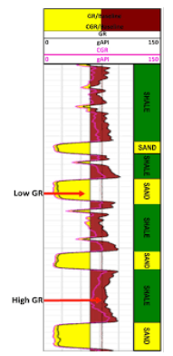
The Gamma Ray log measures the natural radioactivity of the formation, mainly emitted by clay and shale minerals. It is used primarily for lithology differentiation, estimating shale volume, and correlating between formations.
Interpretation guidelines:
High GR values indicate clay-rich or shale intervals.
Low GR values point to cleaner formations (such as sandstone or carbonate) with lower clay content.
As a rule of thumb, for clean sand or carbonate, you might see GR values below ~50 API, while shale-rich zones may exceed ~100 API (though specific numbers depend on local baseline).
Rapid fluctuations or a jagged GR curve can suggest thin-beds or alternating layers of sand and shale.
Use GR as a first-pass indicator of clean versus dirty zones.
2.2 Resistivity (Deep/Medium/Shallow)
Resistivity logs measure how strongly the formation resists the flow of electrical current. The response depends on the Formation's Porosity, fluid content, and salinity of the formation fluids.
Interpretation guidelines:
A high resistivity reading in a porous interval often implies hydrocarbon presence (since oil/gas are less conductive than saline water).
A low resistivity reading typically indicates water-filled pores or a conductive formation (high salinity fluid).
The differences between shallow, medium, and deep resistivity tools help assess mud-filtrate invasion and estimate true formation resistivity.
For example, in a low-GR zone (clean formation), if you see deep Resistivity > ~20 ohm-m, this might suggest hydrocarbons; whereas < ~5 ohm-m could indicate water saturation. But Resistivity alone does not tell the full story; it must be cross-checked with porosity and lithology information.

2.3 Density Logging (RHOB)
The Density log (often noted as RHOB) measures the bulk density of the formation (including matrix rock and pore fluids) using gamma-ray scattering or neutron/gamma interactions.
It is used to calculate Porosity when matrix and fluid densities are known or assumed.
It also helps in lithology discrimination: denser rocks (e.g., carbonates) will give higher density readings than less dense rocks (e.g., many sandstones).
2.4 Neutron Porosity (NPHI)
The Neutron Porosity log measures the hydrogen content in the formation. Since hydrogen atoms are largely contained in pore fluids (e.g., water or hydrocarbons), the hydrogen index provides a proxy for fluid volume in the pores.
When paired with the density log, the neutron log helps estimate Porosity.
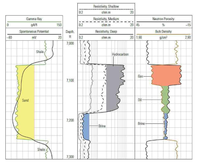
In gas zones, you may observe a "crossover" effect: the neutron porosity reads lower than the density porosity because gas contains fewer hydrogen atoms.

Porosity interpretation from Density & Neutron logs
Density porosity (φ_d) = (ρ_matrix – ρ_bulk) / (ρ_matrix – ρ_fluid) where ρ_matrix is known, ρ_fluid is assumed.
Neutron porosity measures hydrogen content, hence fluid volume in pores; it is often paired with density for more accurate results.
A good reservoir typically has porosity above ~15% (varies by play).
In gas zones, you may see a crossover: neutron reads lower than density (because gas has less hydrogen).
2.5 Sonic (Acoustic) Transit Time (DT)
The Sonic tool measures the travel time of acoustic (compressional) waves through the formation: slower wave velocity (i.e., higher transit time) generally corresponds to more porous or fluid-filled rock.
The sonic log can be used to estimate Porosity.
It also provides mechanical information (e.g., formation compaction, brittleness) and can indicate the presence of fractures or vugs via anomalies in the log trace.

2.6 Spontaneous Potential (SP)
The SP log measures the natural voltage difference between the formation and the borehole fluid. It primarily works in conductive mud systems (e.g., water-based mud) and is less reliable in non-conductive mud systems (e.g., oil-based mud).
It aids in identifying permeable zones (e.g., sands versus shales).
It can also help estimate formation water resistivity or correlate zone continuity.

2.7 Caliper Log
The Caliper log records the borehole diameter (or deviations from the nominal size) and is critical for assessing borehole condition:
Detects borehole enlargement or washout.
Helps correct or flag other logs (density, neutron, sonic) where tool contact or borehole conditions are poor.
If the caliper indicates a significant washout, you must interpret other logs cautiously or discard unreliable intervals.

2.8 NMR (Nuclear Magnetic Resonance) Logging
NMR logging directly assesses pore-size distribution, free versus bound fluid types, and can provide a better permeability estimate in complex reservoirs (e.g., vuggy carbonates, tight sands).
Key outputs: Free Fluid Index (FFI) – easily producible fluid, Bound Fluid Index (BFI) – fluid trapped in small pores.
Use NMR data where available to resolve ambiguous zones or refine reservoir quality.

2.9 LWD/MWD Logging-While-Drilling
Although many of the above tools are wireline, LWD and MWD sensors provide similar or proxy measurements while drilling, enabling real-time or near-real-time decisions. These are especially valuable for steering, casing decisions, and for early formation evaluation.
3. Combination of Logs – Integrating for Robust Interpretation
Using each log independently provides insight, but the real value lies in combining tool responses in a workflow. Below are typical field workflows that drilling professionals can apply.
3.1 GR + SP tracks for initial lithology & fluid indication
Use the GR log to identify clean vs shaly zones (clean sands/carbonates vs clays).
In a conductive mud scenario, look at SP: if the GR shows a low baseline (clean zone) and SP deflects significantly, this may indicate a permeable sand.
This "scan" is useful early in logging to flag intervals of interest while drilling or during logging operations.
3.2 Neutron-Density overlay (Gas / Porosity-check)
Overlay the Neutron and Density porosity logs on the same track.
If the two curves track closely together (i.e., overlap), it suggests that the pore fluid is liquid (water or oil) and that the formation is homogeneous.
Suppose the density porosity is significantly higher than the neutron porosity (i.e., neutron reads lower). In that case, this is the classic "crossover" gas effect (because of fewer hydrogen atoms in the gas), a strong gas indication.
After that, take an average (or appropriate weighted combination) of the two to estimate Porosity (unless gas effect or other anomalies require correction).

3.3 Resistivity + Porosity + Shale Volume for Water Saturation (Sₙ)
After lithology and Porosity are reasonably assessed:
Use Resistivity (corrected for invasion) to estimate true formation resistivity (Rₜ).
Estimate formation water resistivity (Rₙ) from offset data or mud log.
Determine Porosity (φ) and shale volume (V_sh) from GR, neutron, density, etc.
Apply the empirical relation (e.g., Archie's law) to compute water saturation: Sw=(a⋅Rwϕm⋅Rt)1/n, where a, m, and n are empirical constants.
In the field, you may not compute full saturation, but apply the logic: good Porosity + low shale + high Resistivity → likely hydrocarbon-bearing zone.
3.4 Image/Caliper + Other Logs for Fracture, Borehole Condition & Geosteering
Use caliper + image logs (if available) to assess borehole condition: washouts, rugosity, tool contact.
Image logs help identify fractures, bedding planes, or vugs, which can influence drilling decisions or completions.
In directional/horizontal wells (especially with LWD), imaging can support geosteering into better formation.
For completions, image logs help identify natural fractures or structural features ideal for perforation or stimulation placement.
3.5 Putting It All Together: Workflow for a Field Interpretation
Here's a streamlined workflow drilling professionals can adopt:
Perform a visual rapid scan: start with GR and identify clean vs. shaly intervals.
Check porosity logs (density/neutron/sonic) for intervals with meaningful Porosity.
Check Resistivity: Does a high resistivity correlate with low GR and good Porosity?
Assess lithology: What formation type are you in (sandstone, carbonate, shale)?
Apply basic saturation logic: clean lithology + good porosity + high resistivity + low shale = candidate pay zone.
Check borehole condition and tool reliability: Caliper for washout, shallow vs deep Resistivity for invasion.
Note any anomalies: neutron/density crossover (gas), image log fractures, borehole enlargement, tool mis-readings.
Label intervals: reservoir interval(s), transition zones, non-pay/shale zones. Use this to guide drilling decisions, casing plans, and completion targets.
4. Deducing Formation Types & Reservoir Properties
Here, we describe how typical log signatures map to common formation types and how to estimate reservoir properties in the field.
4.1 Formation Types
Sandstone
GR: low (if clean sand) unless it is shaly.
Density: moderate (for quartz ~2.65 g/cc) unless significant matrix variations or fluid effect.
Neutron: shows Porosity; density-neutron overlay often close unless gas present.
Resistivity: variable, high if hydrocarbon-bearing, low if water-saturated.
Sonic: moderate transit time.
Field clue: Low GR + moderate density + good Porosity + high Resistivity = sandstone reservoir candidate.
Carbonate (Limestone / Dolomite)
GR: very low (typically) due to low clay content.
Density: higher values (e.g., dolomite ~2.87 g/cc, limestone ~2.71 g/cc) → the density log will respond accordingly.
Neutron: depends on pore type and whether vugs/fractures are present, can read high or low.
Sonic: In vuggy or fractured carbonates, you may see slower wave velocities (longer transit times).
Resistivity: again depends on fluid content.
Field clue: Very low GR + high density + possible sonic slowdown or high porosity indication + favourable porosity/resistivity = carbonate reservoir candidate.
Shale / Clay-Rich Formation
GR: high, reveals large clay or shale content.
Neutron: high (because of hydrogen in bound water in clay).
Resistivity: low (saline water in clay, conductive matrix).
Density: often moderate to low (clays generally less dense than carbonates).
Field clue: High GR + low Resistivity + high neutron + poor Porosity = low reservoir quality zone.
4.2 Reservoir Property Estimation
Porosity (φ)
Neutron porosity is derived from hydrogen content and is often averaged with density porosity unless gas or other anomalies require correction.
Effective Porosity = total Porosity minus bound water/shale pores, etc.
Field guideline: A "good" reservoir usually has Porosity > ~15% (depending on play, geology, and economic threshold).
Permeability (k) – Field Estimate
Conventional logs do not measure permeability directly, but you can infer trends: higher Porosity + good connectivity (low shale volume) + presence of fractures → likely higher permeability.
In more advanced workflows (or with NMR/sonic), you can derive better permeability estimates. For example: k=100×ϕ2×(1−Swirr)Swirr, Where S_wirr is irreducible water saturation.
In the field, focus on the "good porosity + low shale + fractures" combination as a practical permeability indicator.
Water Saturation (Sₙ)
As discussed in Section 3.3, use Resistivity + Porosity + shale volume via Archie's or modified equations.
Field shorthand: Clean lithology + good Porosity + high Resistivity = low water saturation → likely hydrocarbon bearing.
Another practical check: if shallow resistivity ≈ deep resistivity → minimal invasion → more reliable Rₜ reading.
Effective Reservoir Thickness / Net Pay
Define intervals where: GR is low (clean), Porosity above threshold (say > ~15 %), resistivity high, shale volume low.
Sum the thickness of those intervals → net pay.
Use net pay and porosity/resistivity data for reserve estimation or well/casing/completion design.
Borehole Invasion & Tool Condition Corrections
Mud filtrate invasion will affect shallow Resistivity; if shallow "deep Resistivity, suspect invasion.
Borehole washouts (seen on caliper) affect log accuracy (density tool may read lower, neutron tool may read higher because of poor contact). Always flag and correct or exclude suspect data.
Use logs as guidance, not absolute truth. Always validate with mud log, cuttings, and cores (if available).
5. Field Applications & Best Practices for Drilling Professionals
This section highlights how drilling operations teams can apply these workflows and integrate log interpretation into day-to-day decisions.
5.1 Real-Time Decision Making While Drilling
Monitor the LWD GR curve as an early indicator: steer toward intervals exhibiting low GR (target sands or carbonates).
Where available, monitor LWD/MWD porosity and resistivity proxies to adjust well trajectory, casing points, and mud programmes.
If image logs indicate upcoming fractures or high-porosity intervals, anticipate changes in drilling parameters (mud weight, bit selection, rate of penetration) and in completion readiness.
5.2 Risk Management – Borehole Conditions
Run caliper logs early, or monitor borehole diameter to identify washouts, rugose hole sections, or zones of poor hole stability.
If borehole conditions are poor, log quality and thus interpretation reliability drop; adjust drilling practices (mud weight, solids control, bit selection) to protect data integrity.
Preventing misinterpretation begins with high-quality holes.
5.3 Completion Planning
Use image logs (if available) to locate natural fractures or bedding planes—these may serve as optimal locations for perforation or stimulation.
Use the interpreted net pay, Porosity, and saturation data to determine perforation intervals, stimulation plans, or sand-screen placements.
Integrate log interpretation into completion design early (e.g., packer placement, zonal isolation, inflow control).
5.4 Troubleshooting & Validation
If logs appear anomalous (for example, density porosity > neutron porosity drastically without a clear gas indication), suspect borehole washout, poor tool contact, or tool malfunction.
In zones of invasion (shallow Resistivity diverges significantly from deep), treat resistivity readings cautiously or use only deeper log readings.
Always cross-check log interpretation against nearby wells (offset logs), core descriptions, cuttings, and mud logs for lithology / fluid consistency.
5.5 Field Checklist Before Interpretation
Verify that tools are calibrated, zero-offsets are checked, and known baselines (clean sand, shale) are established.
Confirm borehole size (via caliper) and mud condition (type, Resistivity). Note if mud is oil-based (SP may not work reliably) or water-based.
Confirm depth alignment of logs and correlate with drilling bit record (depths, hole sections).
Mark initial intervals of interest (low GR, high Resistivity, good Porosity) for follow-up detailed petrophysical interpretation later.
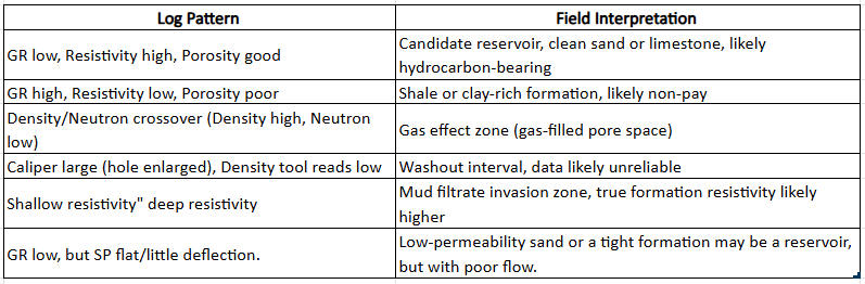
6. Quick Cheat-Sheet for Field Interpretation
7. Summary
This guide equips drilling professionals with a structured and clear approach to log interpretation in the field:
Understand what each log tool measures and how to interpret its output.
Combine logs (lithology + Porosity + Resistivity + borehole checks) to strengthen your interpretation.
Deduce formation types (sandstone, carbonate, shale) and estimate key reservoir properties (Porosity, saturation, permeability).
Use practical field workflows and checklists to support real-time decisions and avoid common pitfalls.
Always assess borehole conditions and tool reliability, and validate your interpretation with ancillary data (mud logs, cores, offset wells).
By applying these practices, you will turn raw log curves into actionable insights, steering wells into favorable zones, avoiding non-productive intervals, designing completions more effectively, and supporting safe, efficient drilling operations.
References
Asquith, G., and Krygowski, D. 2004. Basic Well Log Analysis, 2nd ed. AAPG Methods in Exploration Series 16. American Association of Petroleum Geologists, Tulsa, Oklahoma.
Rider, M.H., and Kennedy, M. 2011. The Geological Interpretation of Well Logs, 3rd ed. Rider-French Consulting Ltd., Sutherland, Scotland.
Serra, O. 1984. Fundamentals of Well-Log Interpretation, Vol. 1: The Acquisition of Logging Data; Vol. 2: Interpretation of Logging Data. Elsevier, Amsterdam, Netherlands.
Hilchie, D.W. 1982. Applied Openhole Log Interpretation. D.W. Hilchie, Inc., Golden, Colorado.
Ellis, D.V., and Singer, J.M. 2007. Well Logging for Earth Scientists, 2nd ed. Springer, Dordrecht, Netherlands.
Crain, E.R. 2023. Crain's Petrophysical Handbook. Accessed October 2025. https://www.spec2000.net
Schlumberger. 2013. Log Interpretation Charts. Schlumberger Oilfield Services, Houston, Texas.
Society of Petroleum Engineers (SPE). 2020. Petroleum Engineering Handbook, Volume V: Reservoir Engineering and Petrophysics. SPE, Richardson, Texas.
Doveton, J.H. 1994. Geological Logging and Well Log Analysis. Society of Petroleum Engineers, Richardson, Texas.
Schlumberger Oilfield Glossary. Formation Evaluation and Logging Tools Sections. Accessed October 2025. https://www.glossary.oilfield.slb.com
U.S. Geological Survey (USGS). 2019. Introduction to Geophysical Well Logging. Public domain educational diagrams. Accessed October 2025. https://pubs.usgs.gov
Crain, E.R. 2023. Crain's Petrophysical Handbook - Log Examples and Crossplots. Accessed October 2025. https://www.spec2000.net
Contains freely usable schematic log examples and generic crossplots (non-commercial use permitted with attribution).Schlumberger Oilfield Glossary (Illustrations Section). Accessed October 2025. https://www.glossary.oilfield.slb.com
Provides open-access schematic diagrams of logging tools and generic log responses under Creative Commons license.Wikimedia Commons (Petrophysics and Well Logging Category). Accessed October 2025. https://commons.wikimedia.org/wiki/Category:Well_logging
Contains Creative Commons–licensed diagrams (e.g., GR-resistivity overlays, SP curves, neutron-density crossovers).Society of Petroleum Engineers (SPE). 2020. Petrophysics Discipline Knowledge Resource. SPE.org.
Some figures in the SPE Learning Center are open for educational use with proper citation.OpenGeoscience, Geological Society of London. Geological Applications of Wireline Logs - Open Figures. Accessed October 2025. https://www.geolsoc.org.uk/opengeoscience